Artificial Neural Networks (ANNs)

Artificial Neural Networks are models inspired by the human brain.
They are made up of layers of simple computing units called neurones, which learn to recognise patterns through training.

Neural networks form the foundation of deep learning, the technology behind computer vision, voice recognition, and language models.

Basic Neurone

A neurone takes several inputs, multiplies each by a weight, adds a bias, and passes the result through a nonlinear function (called an activation function).

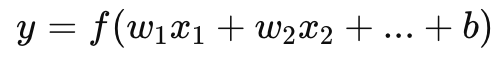
Where:

• x₁, x₂, ... = inputs
• w₁, w₂, ... = weights (learned parameters)
• b = bias term
• f = activation function (e.g., sigmoid, ReLU)

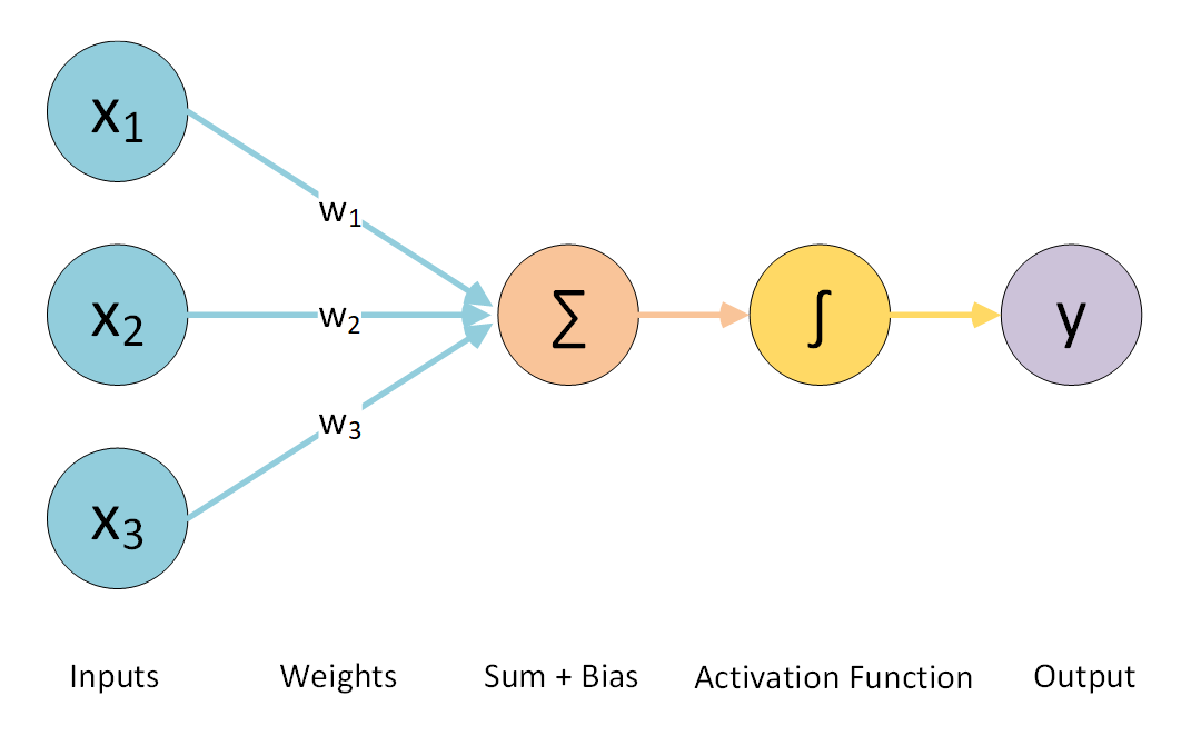
So there can be any number of inputs and the inputs can be any value. Each input is multiplied by its weight, and then all these totals are summed together and a bias is added to it. This then gets fed in to the activation function to generate an output value for that neurone. As networks are trained, the weights on each input and the neurones bias value are adjusted each cycle, these are the learned parameters for the neurone.

The input values, while they can be any value, they are often normalised or scaled to help training. This isn't required, but can make training faster, more stable and less likely to get stuck.

Network Architecture

A neural network typically has:

1. Input layer – receives the data features.
2. Hidden layers – transform inputs through neurones.
3. Output layer – produces final predictions, e.g. class probabilities.

Each neurone in a layer connects to neurones in the next layer.

Activation Functions

Activation functions introduce nonlinearity, allowing networks to learn complex patterns.

If a neural network used only linear operations, then no matter how many layers it had, the whole system would still behave like a single linear classifier. That means it could only draw a straight line to separate classes.

But real-world data is rarely separable by a straight line.
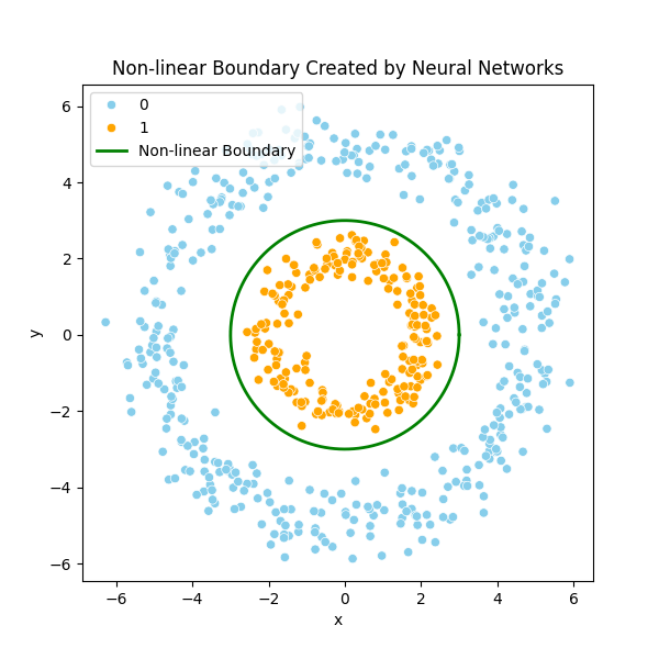
For example, imagine a dataset where one class forms a tight circle inside another class. A straight line can’t separate the inner points from the outer ones.

Activation functions introduce non-linearity, which lets the network bend, twist, and combine many small curves to form complex decision boundaries.
Instead of one straight line, the network can create an irregular closed shape that perfectly wraps around the inner cluster.
This is what gives neural networks their expressive power.

Example

Here you can see two clusters plotted on a scatter chart:

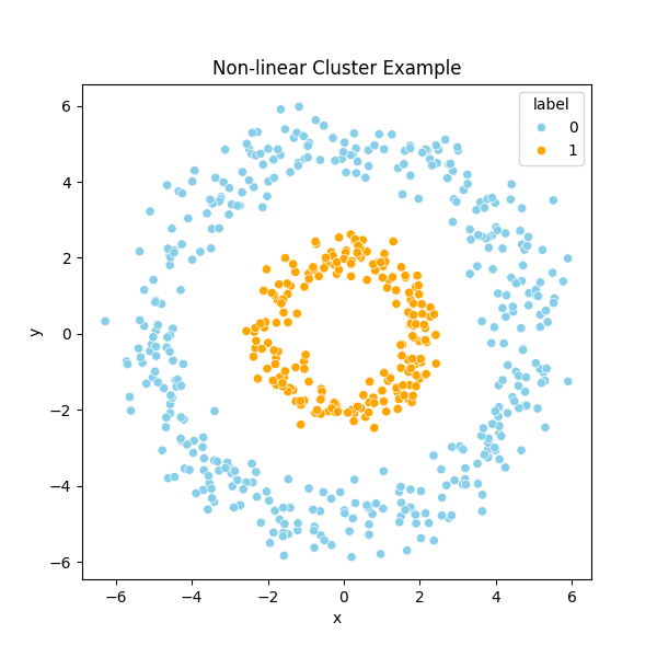
If you tried to use a linear approach then there is no line that you can draw that separates the clusters and give you good results:

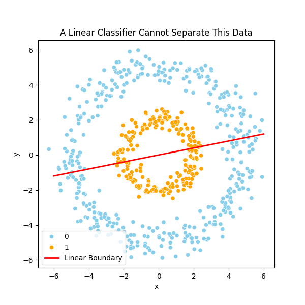
However, using neural networks with activation functions, you can separate clusters with a lot more detailed, irregular shaped, line that is made up with many small curves. This allows you to properly identify clusters (the example image is a circle but in reality can be any irregular shape):

Some common activation functions

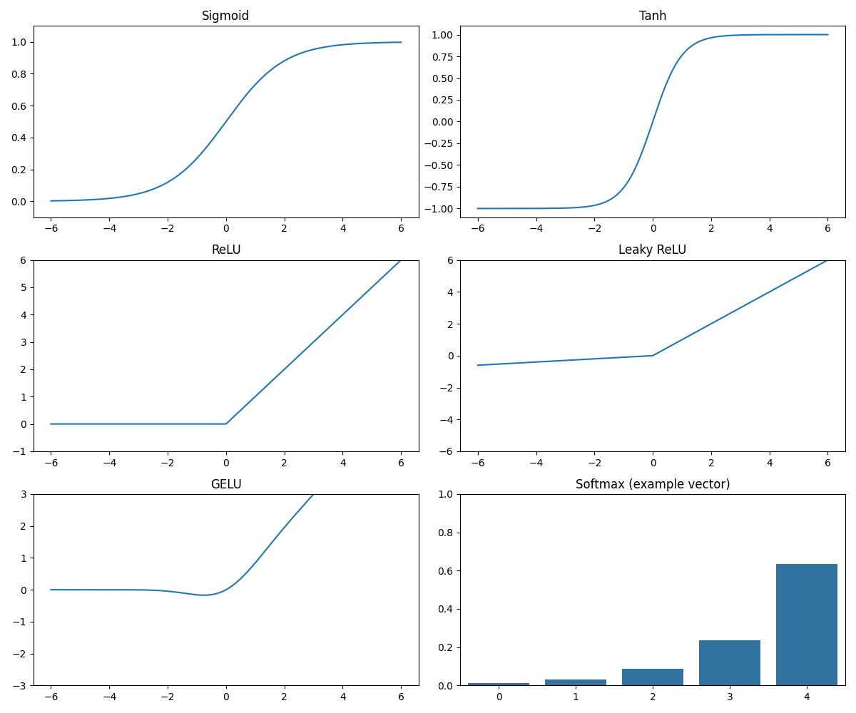
Charts displaying the shape of different activation functions

When to use each activation?

Implementing a Simple Neural Network with Keras

We’ll use Keras, a high-level library built on top of TensorFlow, to train a simple ANN on a classic dataset.

Example Classifying Iris Flower Species:

Output:

Explanation:

• Each Dense layer connects all neurons from one layer to the next.
• relu activation allows complex nonlinear learning.
• softmax converts the last layer’s outputs into probabilities that sum to 1.
• We train for 50 “epochs” — one full pass over the training data.
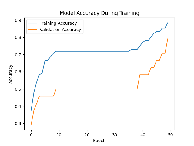
• The history object stores accuracy and loss per epoch for visualisation.

Understanding Model Output

After training, you can use the model to make predictions:

Output:

Explanation:

• The model outputs 3 probability scores (for each species).
• The class with the highest probability is selected as the prediction.

Preventing Overfitting

Overfitting happens when the model performs very well on training data but poorly on new data.
You can reduce overfitting by:

• Using validation sets (like validation_split)
• Applying Dropout layers
• Collecting more data
• Using early stopping (stop training when validation loss stops improving)

Example: adding a dropout layer