Core Algorithms: Clustering and Trees

Machine Learning Fundamentals with Python

3 min read

Published Nov 16 2025

ClusteringImagesK-MeansLinear RegressionLogistic RegressionMachine LearningNeural NetworksNLPNumPyPythonRandom Forestsscikit-learnSupervised LearningUnsupervised Learning

In this section, you’ll learn two very different yet essential approaches in machine learning:

How to group similar data points automatically (K-Means Clustering).
How to make decisions and predictions using tree-based models.

K-Means Clustering (Unsupervised Learning)

K-Means is a simple and powerful unsupervised algorithm that groups data points into K clusters.
Each cluster is defined by its centroid (the average position of all points in that group).

It works like this:

Choose the number of clusters (K).
Randomly place K centroids.
Assign each data point to the nearest centroid.
Move each centroid to the mean of its assigned points.
Repeat until the centroids stop moving (converge).

Example: Clustering Customers by Spending Behaviour

import numpy as np

import pandas as pd

from sklearn.cluster import KMeans

import matplotlib.pyplot as plt

# Example data: [Annual Income (k£), Spending Score (1–100)]

data = {

'Annual_Income': [15, 16, 17, 18, 19, 20, 21, 22, 23, 24],

'Spending_Score': [39, 81, 6, 77, 40, 76, 10, 94, 12, 90]

}

df = pd.DataFrame(data)

# Create a KMeans model

kmeans = KMeans(n_clusters=2, random_state=42)

kmeans.fit(df)

# Add cluster labels to the dataset

df['Cluster'] = kmeans.labels_

print(df)

# Plot the clusters

plt.scatter(df['Annual_Income'], df['Spending_Score'], c=df['Cluster'], cmap='viridis')

plt.scatter(kmeans.cluster_centers_[:, 0], kmeans.cluster_centers_[:, 1],

color='red', marker='X', s=200, label='Centroids')

plt.xlabel("Annual Income (k£)")

plt.ylabel("Spending Score")

plt.title("K-Means Clustering Example")

plt.legend()

plt.tight_layout()

plt.show()

Output:

Annual_Income Spending_Score Cluster

0 15 39 1

1 16 81 0

2 17 6 1

3 18 77 0

4 19 40 1

5 20 76 0

6 21 10 1

7 22 94 0

8 23 12 1

9 24 90 0

machine learning fundamentals k means clustering example

Explanation:

Each customer is represented as a point in 2D space.
The algorithm automatically divides them into two clusters (low spenders vs high spenders).
The red X marks show the cluster centres (averages).

Choosing the Right Number of Clusters (Elbow Method)

We can plot the “inertia” (sum of distances to the nearest centroid) for different K values.
The point where inertia starts to flatten out (the “elbow”) is usually a good choice for K.

inertia_values = []

for k in range(1, 8):

km = KMeans(n_clusters=k, random_state=42)

km.fit(df[['Annual_Income', 'Spending_Score']])

inertia_values.append(km.inertia_)

plt.plot(range(1, 8), inertia_values, marker='o')

plt.xlabel("Number of Clusters (K)")

plt.ylabel("Inertia")

plt.title("Elbow Method for Choosing K")

plt.tight_layout()

plt.show()

machine learning fundamentals k means elbow method

Explanation:

If K = 1, all points are in one big cluster (high inertia).
As K increases, inertia decreases.
After the “elbow,” adding more clusters gives little improvement.

Decision Trees (Supervised Learning)

Decision Trees are supervised models that split data step by step based on feature values.
They ask a sequence of “yes/no” questions to make predictions.

Example:

Is Age > 30?

│

├── Yes → Income > 50k? → Class A

└── No → Class B

Each split tries to make the resulting groups purer — that is, more uniform in their labels.

Example: Predicting if Someone Buys a Product

import pandas as pd

from sklearn.tree import DecisionTreeClassifier, plot_tree

from sklearn.model_selection import train_test_split

from sklearn.metrics import accuracy_score

import matplotlib.pyplot as plt

# Example data

data = {

'Age': [22, 25, 47, 52, 46, 56, 55, 60],

'Income': [25000, 30000, 45000, 50000, 60000, 80000, 70000, 90000],

# 1 = Yes, 0 = No

'Buys': [0, 0, 1, 1, 1, 1, 1, 1]

}

df = pd.DataFrame(data)

X = df[['Age', 'Income']]

y = df['Buys']

# Split data

X_train, X_test, y_train, y_test = train_test_split(X, y, test_size=0.25, random_state=42)

# Train model

tree = DecisionTreeClassifier(max_depth=3, random_state=42)

tree.fit(X_train, y_train)

# Predict

y_pred = tree.predict(X_test)

print("Predictions:", y_pred)

print("Accuracy:", accuracy_score(y_test, y_pred))

# Visualise the tree

plt.figure(figsize=(10,6))

plot_tree(tree, feature_names=['Age', 'Income'], class_names=['No', 'Yes'], filled=True)

plt.title("Decision Tree Example")

plt.tight_layout()

plt.show()

Output:

Predictions: [0 1]

Accuracy: 1.0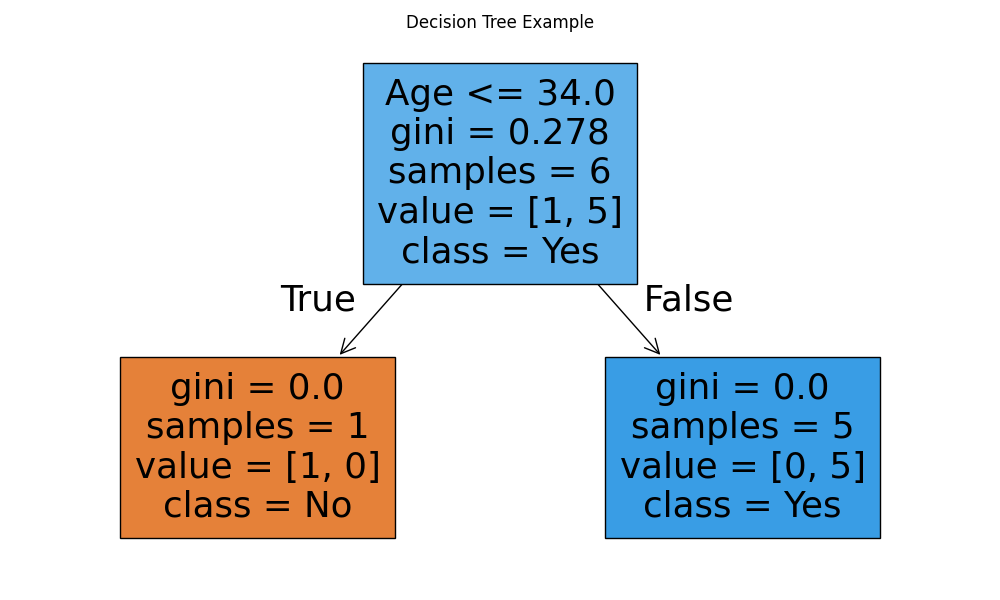

machine learning fundamentals decision tree example

Explanation:

The model finds rules that best separate people who buy vs don’t buy.
The tree’s structure shows how decisions are made.
max_depth controls how deep (complex) the tree can grow.

Random Forests (Many Trees Combined)

A Random Forest is a collection (ensemble) of many decision trees.
Each tree sees a slightly different subset of the data, and their predictions are combined (majority vote).

Benefits:

Reduces overfitting.
Increases accuracy and robustness.
Works well “out of the box.”

Example: Using a Random Forest

from sklearn.ensemble import RandomForestClassifier

from sklearn.metrics import classification_report

# Train a random forest

forest = RandomForestClassifier(n_estimators=100, random_state=42)

forest.fit(X_train, y_train)

# Predict

y_pred = forest.predict(X_test)

print("Accuracy:", accuracy_score(y_test, y_pred))

print("\nClassification Report:\n", classification_report(y_test, y_pred))

Explanation:

n_estimators=100 means we use 100 trees.
Each tree votes, and the majority decision becomes the final prediction.
Random forests handle messy real-world data better than a single tree.

Comparing Clustering and Trees

Aspect	K-Means	Decision Tree / Random Forest
Type	Unsupervised	Supervised
Goal	Group similar data	Predict target labels
Output	Cluster assignments	Class labels / probabilities
Requires labels?	No	Yes
Example	Segmenting customers	Predicting if someone buys