Core Algorithms: Regression

Machine Learning Fundamentals with Python

4 min read

Published Nov 16 2025

ClusteringImagesK-MeansLinear RegressionLogistic RegressionMachine LearningNeural NetworksNLPNumPyPythonRandom Forestsscikit-learnSupervised LearningUnsupervised Learning

Regression is one of the most fundamental concepts in machine learning. It’s all about finding the relationship between variables — specifically, how input features affect an output value.

What Is Regression?

Regression predicts continuous (numeric) outcomes.
Example:

Predicting house prices based on features like size or location.
Predicting sales revenue given advertising spend.
Predicting student scores from hours studied.

Linear Regression – The Basics

Idea:
Fit a straight line (or hyperplane in higher dimensions) that best predicts the target variable.

Formula for simple linear regression:

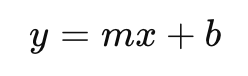
machine learning fundamentals linear regression formula

Where:

y = predicted value
x = input feature
m = slope (coefficient)
b = intercept (bias)

Scikit-learn automatically calculates these for you.

Example: Predicting House Prices:

import numpy as np

import pandas as pd

from sklearn.linear_model import LinearRegression

from sklearn.model_selection import train_test_split

import matplotlib.pyplot as plt

# Sample dataset

data = {

'size_sqft': [1000, 1500, 2000, 2500, 3000],

'price': [200000, 250000, 280000, 310000, 360000]

}

df = pd.DataFrame(data)

# Split into input (X) and output (y)

X = df[['size_sqft']] # features must be 2D

y = df['price']

# Train-test split (just for demonstration)

X_train, X_test, y_train, y_test = train_test_split(X, y, test_size=0.2, random_state=42)

# Create and train model

model = LinearRegression()

model.fit(X_train, y_train)

# Make predictions

y_pred = model.predict(X_test)

# Visualise

plt.scatter(X, y, color='blue', label='Actual')

plt.plot(X, model.predict(X), color='red', label='Predicted line')

plt.xlabel("House Size (sqft)")

plt.ylabel("Price (£)")

plt.title("Linear Regression Example")

plt.legend()

plt.tight_layout()

plt.show()

# Print learned parameters

print("Slope (Coefficient):", model.coef_[0])

print("Intercept:", model.intercept_)

Output:

machine learning fundamentals linear regression example

Slope (Coefficient): 78.28571428571426

Intercept: 121142.85714285719

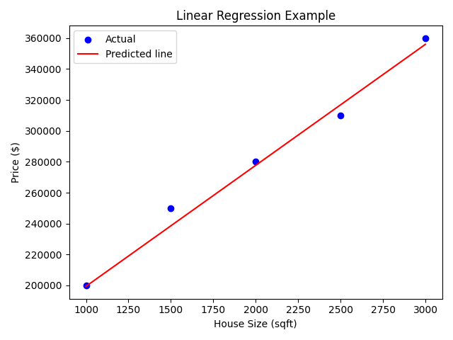
Explanation:

We fitted a straight line that best represents the relationship between house size and price.
The slope tells how much the price increases per additional square foot.
The intercept tells the estimated price when size = 0 (theoretically).

Evaluating Regression Performance

We measure how well a regression model predicts actual values using metrics such as:

MAE (Mean Absolute Error) : Average of absolute errors
- Good values - Small number (close to 0), meaning your predictions are, on average, very close to the actual values.
- - Good depends on the target scale, eg. If house prices are around £300,000, an MAE of £5,000 is great, however, if house prices are around £100, an MAE of £5,000 is awful.
- Bad values - Large number, predictions are far off.
MSE (Mean Squared Error) : Average of squared errors (penalises big mistakes)
- Good values - Small number, often much smaller than the square of your target values.
- Bad values - Large number, indicates large mistakes or many medium-sized mistakes.
RMSE (Root Mean Squared Error) : Square root of MSE (same units as target)
- Good values - Small, relative to typical values in your dataset. RMSE ≈ MAE → errors consistent (good sign).
- Bad values - Large, especially compared to the dataset’s typical values. RMSE > MAE → the model is making occasional very bad mistakes.
R² (Coefficient of Determination) : How much of the variation in the target the model explains.
- Good values - 0.70 – 1.0 → strong predictive power, 1.0 → perfect (rare in real life)
- Bad values - 0.0 → model is no better than predicting the mean, Negative value → model is worse than the baseline.
- Guidelines:
- - > 0.9 → excellent (common in physics, rare in social sciences)
  - 0.6 – 0.8 → solid model
  - 0.3 – 0.6 → fair (useful but not great)
  - 0.0 – 0.3 → weak model
  - < 0 → actively bad model

Example:

from sklearn.metrics import mean_absolute_error, mean_squared_error, r2_score

mae = mean_absolute_error(y_test, y_pred)

mse = mean_squared_error(y_test, y_pred)

rmse = np.sqrt(mse)

r2 = r2_score(y_test, y_pred)

print(f"MAE: {mae:.2f}")

print(f"MSE: {mse:.2f}")

print(f"RMSE: {rmse:.2f}")

print(f"R²: {r2:.2f}")

Logistic Regression – When Outputs Are Categories

Despite the name, logistic regression is used for classification, not regression. It predicts the probability that an input belongs to a certain class (e.g., spam or not spam).

The logistic function (sigmoid) converts linear output into a probability between 0 and 1:

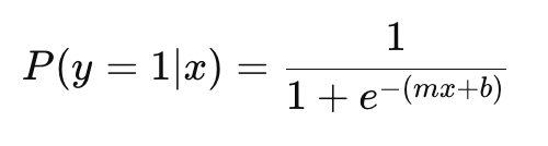
machine learning fundamentals logistic regression formula

If P>0.5, predict 1 (positive class); otherwise 0.

Example: Predicting If a Student Passes an Exam:

import numpy as np

import pandas as pd

from sklearn.linear_model import LogisticRegression

from sklearn.model_selection import train_test_split

from sklearn.metrics import accuracy_score, confusion_matrix, classification_report

# Dataset: hours studied vs. passed (1) or failed (0)

data = {

'hours_studied': [1, 2, 3, 4, 5, 6, 7, 8, 9, 10],

'passed': [0, 0, 0, 0, 1, 1, 1, 1, 1, 1]

}

df = pd.DataFrame(data)

# Features and labels

X = df[['hours_studied']]

y = df['passed']

# Split data

X_train, X_test, y_train, y_test = train_test_split(X, y, test_size=0.3, random_state=42)

# Train model

model = LogisticRegression()

model.fit(X_train, y_train)

# Predict

y_pred = model.predict(X_test)

# get probabilities

y_proba = model.predict_proba(X_test)

print("Predictions:", y_pred)

print("Probabilities:\n", y_proba)

# Evaluate

print("\nAccuracy:", accuracy_score(y_test, y_pred))

print("\nConfusion Matrix:\n", confusion_matrix(y_test, y_pred))

print("\nClassification Report:\n", classification_report(y_test, y_pred))

Output:

Predictions: [1 0 1]

Probabilities:

[[0.01122793 0.98877207]

[0.93724208 0.06275792]

[0.19778737 0.80221263]]

Accuracy: 1.0

Confusion Matrix:

[[1 0]

[0 2]]

Classification Report:

precision recall f1-score support

0 1.00 1.00 1.00 1

1 1.00 1.00 1.00 2

accuracy 1.00 3

macro avg 1.00 1.00 1.00 3

weighted avg 1.00 1.00 1.00 3

machine learning fundamentals logistic regression example

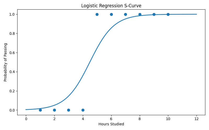
Explanation:

Predictions - these are the model’s final yes/no guesses (1 = pass, 0 = fail) for the students in the test set.
Probabilities - for each student, logistic regression gives two probabilities:
- Column 0 → likelihood of failing
- Column 1 → likelihood of passing
- The prediction (0 or 1) is whichever probability is higher. This shows how confident the model is.
Accuracy - % of test predictions the model got correct.
Confusion matrix - [[TN, FP], [FN, TP]] tells you exactly where mistakes happened:
- TN (true negatives): correctly predicted fails
- FP (false positives): predicted pass but actually failed
- FN (false negatives): predicted fail but actually passed
- TP (true positives): correctly predicted passes
Classification Report - more detailed view than accuracy alone, for each class (0 = fail, 1 = pass):
- Precision: when the model predicts pass/fail, how often is it right?
- Recall: how well the model finds all actual passes/fails
- F1-score: combined measure of precision + recall
- Support: number of true examples of each class

Comparing Linear vs Logistic Regression

Aspect	Linear Regression	Logistic Regression
Output	Continuous numeric value	Probability (0–1)
Used for	Regression problems	Classification problems
Example	Predicting house price	Predicting if an email is spam
Function	Straight line	Sigmoid (S-shaped curve)