Model Evaluation and Performance Analysis

Machine Learning Fundamentals with Python

3 min read

Published Nov 16 2025

ClusteringImagesK-MeansLinear RegressionLogistic RegressionMachine LearningNeural NetworksNLPNumPyPythonRandom Forestsscikit-learnSupervised LearningUnsupervised Learning

Why Evaluate Models?

Building a model is only half the job — the other half is knowing how well it performs.

Evaluation tells us:

How accurate and reliable the model is
Whether it’s overfitting or underfitting
How it might behave on unseen, real-world data

The key principle:

Always evaluate on data your model hasn’t seen before (the test set).

Regression Model Metrics

When your model predicts continuous values (like prices or scores), you can use these metrics:

MAE (Mean Absolute Error) - Average absolute difference between predictions and true values.
MSE (Mean Squared Error) - Average of squared errors (penalises large mistakes).
RMSE (Root Mean Squared Error) - Square root of MSE (same units as target).
R² (Coefficient of Determination) - How much variance in data is explained.

Example: Evaluating a Regression Model

from sklearn.linear_model import LinearRegression

from sklearn.metrics import mean_absolute_error, mean_squared_error, r2_score

from sklearn.model_selection import train_test_split

import numpy as np

import pandas as pd

# Simple dataset: size vs. price

data = {

'size_sqft': [1000, 1500, 2000, 2500, 3000],

'price': [200000, 250000, 280000, 310000, 360000]

}

df = pd.DataFrame(data)

X = df[['size_sqft']]

y = df['price']

X_train, X_test, y_train, y_test = train_test_split(X, y, test_size=0.4, random_state=42)

model = LinearRegression()

model.fit(X_train, y_train)

y_pred = model.predict(X_test)

mae = mean_absolute_error(y_test, y_pred)

mse = mean_squared_error(y_test, y_pred)

rmse = np.sqrt(mse)

r2 = r2_score(y_test, y_pred)

print(f"MAE: {mae:.2f}")

print(f"MSE: {mse:.2f}")

print(f"RMSE: {rmse:.2f}")

print(f"R²: {r2:.2f}")

Output:

MAE: 10714.29

MSE: 115306122.45

RMSE: 10738.07

R²: 0.96

Explanation:

MAE, MSE, and RMSE measure “how far off” predictions are.
R² measures how much of the true variation your model explains.

Classification Model Metrics

When predicting categories e.g. “spam” or “not spam”, accuracy alone can be misleading, especially with unbalanced data.

Key Metrics:

Accuracy - Proportion of correct predictions.
Precision - Of all predicted positives, how many were correct.
Recall - Of all actual positives, how many were found.
F1 Score - Harmonic mean of precision and recall (balances both).
Confusion Matrix - Table showing counts of true/false positives/negatives.

Example: Binary Classification Evaluation

from sklearn.linear_model import LogisticRegression

from sklearn.metrics import accuracy_score, precision_score, recall_score, f1_score, confusion_matrix, classification_report

from sklearn.model_selection import train_test_split

import pandas as pd

# Example dataset

data = {

'hours_studied': [1, 2, 3, 4, 5, 6, 7, 8, 9, 10],

'passed': [0, 0, 0, 0, 1, 1, 1, 1, 1, 1]

}

df = pd.DataFrame(data)

X = df[['hours_studied']]

y = df['passed']

X_train, X_test, y_train, y_test = train_test_split(X, y, test_size=0.3, random_state=42)

model = LogisticRegression()

model.fit(X_train, y_train)

y_pred = model.predict(X_test)

print("Confusion Matrix:\n", confusion_matrix(y_test, y_pred))

print("\nClassification Report:\n", classification_report(y_test, y_pred))

Output:

Confusion Matrix:

[[1 0]

[0 2]]

Classification Report:

precision recall f1-score support

0 1.00 1.00 1.00 1

1 1.00 1.00 1.00 2

accuracy 1.00 3

macro avg 1.00 1.00 1.00 3

weighted avg 1.00 1.00 1.00 3

Explanation:

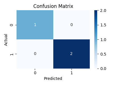
The confusion matrix shows predictions vs actuals, [[TN FP], [FN TP]]:
- TN = True Negative (correctly predicted 0)
- TP = True Positive (correctly predicted 1)
- FP = False Positive (predicted 1 but should be 0)
- FN = False Negative (predicted 0 but should be 1)
The classification report summarises all major metrics.

Visualising Performance with a Confusion Matrix

import seaborn as sns

import matplotlib.pyplot as plt

cm = confusion_matrix(y_test, y_pred)

plt.figure(figsize=(4,3))

sns.heatmap(cm, annot=True, fmt='d', cmap='Blues')

plt.xlabel("Predicted")

plt.ylabel("Actual")

plt.title("Confusion Matrix")

plt.tight_layout()

plt.show()

A heatmap makes it easy to spot where your model is making mistakes (e.g., mixing up similar classes).

machine learning fundamentals confusion matrix

ROC Curves and AUC

The ROC curve (Receiver Operating Characteristic) plots the tradeoff between True Positive Rate (Recall) and False Positive Rate.
The AUC (Area Under the Curve) gives a single measure of overall performance.

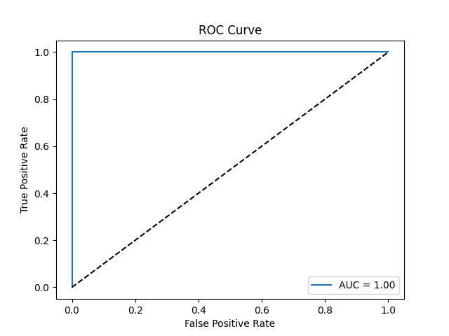
from sklearn.metrics import roc_curve, roc_auc_score

# Get predicted probabilities

y_proba = model.predict_proba(X_test)[:,1]

fpr, tpr, thresholds = roc_curve(y_test, y_proba)

auc = roc_auc_score(y_test, y_proba)

plt.plot(fpr, tpr, label=f'AUC = {auc:.2f}')

plt.plot([0,1], [0,1], 'k--')

plt.xlabel("False Positive Rate")

plt.ylabel("True Positive Rate")

plt.title("ROC Curve")

plt.legend()

plt.show()