Power Law (Pareto) Distribution

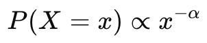
A Power Law Distribution describes a situation where small occurrences are extremely common,
but large occurrences are very rare, following the general rule:

In simple terms:

“A few items account for most of the effect.”
Examples: a few rich people own most wealth, a few websites get most traffic, a few words dominate language use.

It is also known as the Pareto Distribution (after economist Vilfredo Pareto).

Probability Density Function (PDF)

Where:

• x_m​ = minimum possible value (scale parameter)
• α = shape parameter (also called the power law exponent)

The PDF decreases rapidly as x increases — forming a long right tail.

Cumulative Distribution Function (CDF)

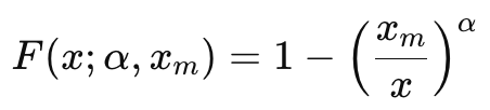
As x → ∞, F(x)→1

Intuition

• Small values are very common (high probability near x_m​)
• Large values are rare, but not impossible — producing a long tail
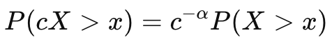
• The distribution is scale-invariant, meaning the shape looks the same at any scale:

Examples

• Wealth distribution - A few individuals hold most wealth
• Internet traffic - Few sites get most visits
• City populations - Few cities are very large
• Word frequencies - Few words used very often
• Social networks - Few users have many followers

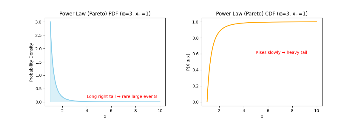
• PDF (left): High probability near the minimum (xₘ), with a long, slow-decaying right tail.
• CDF (right): Increases quickly at first, then slowly approaches 1.

The Power Law shows that extreme events are rare but not negligible.
The tail never fully disappears — there’s always some chance of very large values.

Effect of α (Shape Parameter)

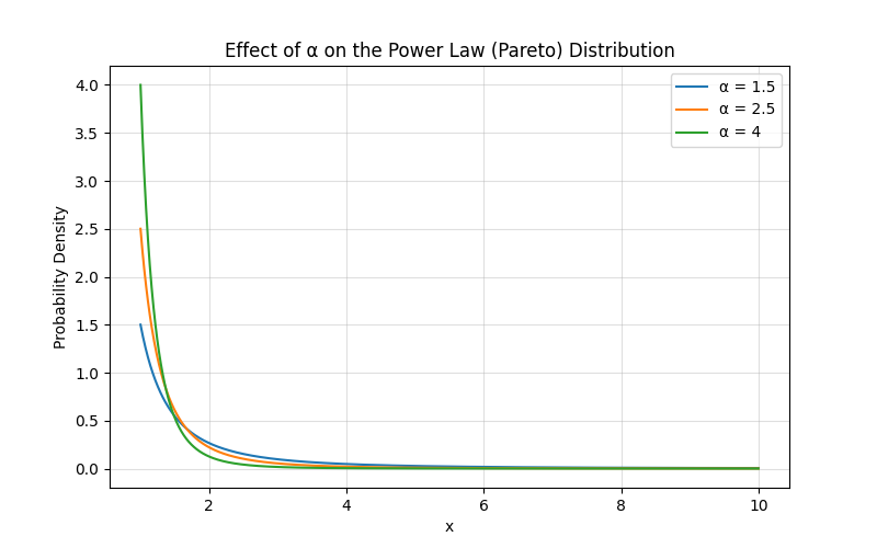
Smaller α → heavier tail (more big events)
Larger α → lighter tail (big events become rarer)

In Machine Learning and Data Science

• Modelling heavy-tailed data - Wealth, web traffic, popularity, network degrees
• Anomaly detection - Detecting rare extreme outliers
• Natural language processing - Word frequencies (Zipf’s law)
• Network science - Power-law degree distributions in social graphs
• Economics / risk modelling - Financial returns, market volatility (tail risk)
• Generative modelling - Sampling realistic “long-tail” distributions