Chart styling

Overall concept

Matplotlib provides two main layers of styling control:

• Global style : Default look for all plots using plt.style.use() or rcParams.
• Figure/Axes-level style : Customisation for one figure or axes using methods like plt.grid(), ax.set_facecolor(), etc.

You can think of it like CSS for charts — global themes + per-element overrides.

Global styles (plt.style)

Matplotlib comes with predefined style sheets that change colours, fonts, gridlines, backgrounds, etc.

import matplotlib.pyplot as plt​# Apply global themeplt.style.use('ggplot')# Examples: 'seaborn', 'dark_background', 'bmh', 'classic', 'Solarize_Light2'

List all available styles:

plt.style.available

Temporarily apply a style:

with plt.style.context('seaborn-v0_8-dark-palette'):    plt.plot([1, 2, 3], [4, 2, 5])    plt.title("Temporarily styled plot")

Exiting the with block restores your default style.

Global customisation via rcParams

Matplotlib’s runtime configuration parameters (rcParams) let you set defaults globally:

plt.rcParams['figure.figsize'] = (8, 6)plt.rcParams['axes.facecolor'] = 'whitesmoke'plt.rcParams['axes.edgecolor'] = 'gray'plt.rcParams['axes.grid'] = Trueplt.rcParams['grid.linestyle'] = '--'plt.rcParams['grid.color'] = 'lightgray'plt.rcParams['font.size'] = 12plt.rcParams['axes.titlesize'] = 14plt.rcParams['axes.labelsize'] = 12

You can also reset them:

plt.rcdefaults()

Figure-level styling

The figure is the overall canvas, so you can control global visual aspects:

fig = plt.figure(figsize=(8, 5), facecolor='white', edgecolor='black')

Example figure-level attributes:

• figsize = Width × height in inches eg. (8, 6)
• facecolor = Background colour of canvas eg. 'white'
• edgecolor = Outline colour of canvas eg. 'black'
• dpi = Resolution (dots per inch) eg. dpi=120

Axes-level styling

Axes are the “plot area” inside the figure — you can adjust their background, borders, ticks, and gridlines:

fig, ax = plt.subplots()​# Background colorax.set_facecolor('whitesmoke')​# Set the grid styleax.grid(True, color='lightgray', linestyle='--', linewidth=0.7)​# Hide top borderax.spines['top'].set_visible(False)​# Hide the right borderax.spines['right'].set_visible(False)​# Set the tick styleax.tick_params(colors='gray', direction='out')​# Add ttitle and labelsax.set_title("Styled Axes", fontsize=14, color='navy')ax.set_xlabel("X Axis", fontsize=12)ax.set_ylabel("Y Axis", fontsize=12)

Gridlines

You can add and style gridlines easily:

 # Turn on gridplt.grid(True)​plt.grid(color='gray', linestyle='--', linewidth=0.5, alpha=0.7)

or at the axes level:

ax.grid(True, axis='y', linestyle=':', color='lightgray')

Styling options:

• axis = 'x', 'y', 'both' eg. axis='x'
• color = Grid colour eg. 'lightgray'
• linestyle = Line pattern wg. '--', ':', '-.'
• linewidth = Thickness eg. 0.5
• alpha = Transparency eg. 0.7

Fonts, titles, and text

Global font settings:

plt.rcParams['font.family'] = 'serif'plt.rcParams['font.size'] = 11

Custom per-plot:

plt.title("Sales by Year", fontsize=16, fontweight='bold', color='navy')plt.xlabel("Year", fontsize=12)plt.ylabel("Revenue ($M)", fontsize=12)

Add text annotation

plt.text() - Places text at a specific (x, y) coordinate in data space.

plt.text(x, y, 'Your text', fontsize=12, color='r', ha='center', va='bottom')

Parameters:

• x, y: Position in the same coordinate system as your plot.
• 'Your text': The string to display.
• fontsize: Font size.
• color (or c): Text colour.
• ha, va: Horizontal and vertical alignment ('left', 'center', 'right', 'top', 'bottom').

Example:

import matplotlib.pyplot as plt​plt.plot([1, 2, 3], [2, 3, 5])plt.text(x=2, y=3, s='Peak point', fontsize=12, color='red')plt.show()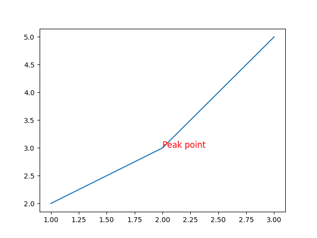

Add a horizontal line

plt.axhline() - Draws a horizontal line across the entire plot (at a specific y-value).

plt.axhline(y=VALUE, color='color', linestyle='--', linewidth=2)

Parameters:

• y: The y-coordinate where the line should appear.
• color (or c): Line colour (e.g. 'red', 'k' for black).
• linestyle: Line pattern ('-', '--', ':', '-.').
• linewidth (or lw): Thickness of the line.
• xmin, xmax: Optional range (0 to 1, fraction of x-axis range).

Example:

import matplotlib.pyplot as plt​plt.plot([1, 2, 3], [2, 3, 5])plt.axhline(y=3, color='r', linestyle='--', label='Target Line')plt.legend()plt.show()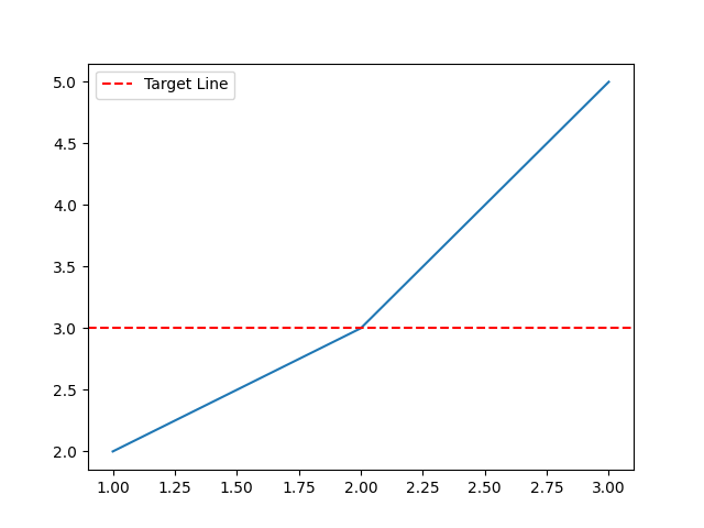

Add a vertical line

plt.axvline() - Draws a vertical line at a specific x-value.

plt.axvline(x=VALUE, color='color', linestyle='--', linewidth=2)

Parameters:

• x: The x-coordinate for the line.
• Other options (color, linestyle, linewidth, ymin, ymax) work just like in axhline().

Example:

import matplotlib.pyplot as plt​plt.plot([1, 2, 3], [2, 3, 5])plt.axvline(x=2, color='g', linestyle='-.', label='Reference Line')plt.legend()plt.show()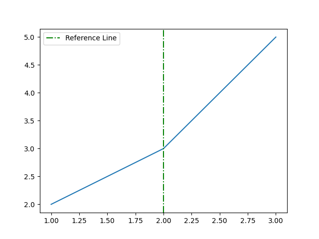

Tick styling

Tweak tick marks and labels:

ax.tick_params(axis='x', colors='gray', direction='out', rotation=45)ax.tick_params(axis='y', colors='gray', labelsize=10)

Hide or customise tick labels:

ax.set_xticks(range(5))ax.set_xticklabels(['A','B','C','D','E'], rotation=30)

Legends

plt.legend(loc='upper left', frameon=False)

Common legend options:

• loc = 'upper left', 'lower right', etc.
• frameon = Show/hide border
• fontsize = Legend text size
• title = Add a title to the legend
• ncol = Columns in legend layout

Creating your own style

For a consistent professional look across projects:

1. Pick a base style (plt.style.use('seaborn-v0_8'))
2. Customise with a few rcParams
3. Save it as your own style file

Create your own style:

plt.style.use('default')plt.rcParams.update({    'axes.facecolor': 'whitesmoke',    'grid.color': 'lightgray',    'axes.edgecolor': 'gray',    'axes.grid': True,    'font.size': 11,})plt.style.use('my_custom_style.mplstyle')

You can store .mplstyle files in your Matplotlib config folder.