Model Evaluation and Validation

Scikit-learn Basics

4 min read

Published Nov 17 2025, updated Nov 19 2025

ClusteringFeature EngineeringK-MeansLinear RegressionLogistic RegressionMachine LearningNumPyPythonRandom Forestsscikit-learnSupervised LearningUnsupervised Learning

Building a model is only half the battle, the other half is knowing how well it actually works.
Model evaluation and validation help ensure that your model’s performance reflects true generalisation, not just how well it memorised the training data.

In Scikit-learn, evaluation and validation are integral parts of the machine-learning process.

You’ll use them to:

Measure predictive performance with metrics
Detect and prevent overfitting
Compare models objectively
Tune hyperparameters confidently

The Importance of Validation

When training a model, it’s easy to overestimate performance if you test it on the same data it was trained on.
This is called overfitting — the model fits the training data too closely and fails on unseen examples.

Two Key Concepts:

Training Error: How well the model fits the data it learned from.
Generalisation Error: How well it performs on new, unseen data.

Goal:

Minimise generalisation error — not just training error.
To estimate generalisation, we reserve a validation set or use cross-validation to simulate multiple training/testing cycles.

Train / Test Split

The simplest validation strategy is to divide the data into training and testing subsets.

from sklearn.model_selection import train_test_split

from sklearn.datasets import load_iris

from sklearn.ensemble import RandomForestClassifier

from sklearn.metrics import accuracy_score

X, y = load_iris(return_X_y=True)

X_train, X_test, y_train, y_test = train_test_split(

X, y, test_size=0.3, random_state=42

)

model = RandomForestClassifier(random_state=42)

model.fit(X_train, y_train)

y_pred = model.predict(X_test)

print("Accuracy:", accuracy_score(y_test, y_pred))

Notes:

test_size=0.3 reserves 30% of data for testing.
random_state ensures reproducibility.
For classification, use stratify=y to maintain class proportions.

While simple, a single split can be misleading if data is small or randomly unbalanced. That’s where cross-validation helps.

Cross-Validation (CV)

Cross-validation gives a more reliable estimate of model performance by splitting the data multiple times and averaging the results.

k-Fold Cross-Validation

Data is divided into k equal parts (“folds”):

Train on k−1 folds
Test on the remaining fold
Repeat k times so each fold is used once as test data

Scikit-learn automates this with cross_val_score.

Example:

from sklearn.model_selection import cross_val_score

from sklearn.svm import SVC

from sklearn.datasets import load_iris

X, y = load_iris(return_X_y=True)

model = SVC(kernel='linear')

scores = cross_val_score(model, X, y, cv=5)

print("Cross-validation scores:", scores)

print("Mean accuracy:", scores.mean())

Output:

Cross-validation scores: [1. 0.93 0.97 0.97 1. ]

Mean accuracy: 0.974

Notes:

cv=5 → five-fold CV (default for many functions).
Results are more robust because they average performance across splits.
Use stratified CV for classification to preserve class ratios.

Stratified K-Fold (for classification)

from sklearn.model_selection import StratifiedKFold, cross_val_score

from sklearn.linear_model import LogisticRegression

from sklearn.svm import SVC

from sklearn.datasets import load_iris

X, y = load_iris(return_X_y=True)

model = SVC(kernel='linear')

cv = StratifiedKFold(n_splits=5, shuffle=True, random_state=42)

model = LogisticRegression(max_iter=200)

scores = cross_val_score(model, X, y, cv=cv)

print("Stratified CV scores:", scores)

print("Mean:", scores.mean())

Stratification prevents bias when class distributions are uneven, essential for imbalanced datasets.

Classification Metrics

Metric	Description	Scikit-learn Function
Accuracy	Fraction of correct predictions	`accuracy_score`
Precision	True positives / (True + False Positives)	`precision_score`
Recall (Sensitivity)	True positives / (True + False Negatives)	`recall_score`
F1 Score	Harmonic mean of precision & recall	`f1_score`
ROC-AUC	Area under the ROC curve	`roc_auc_score`

Example:

from sklearn.metrics import precision_score, recall_score, f1_score, confusion_matrix

print("Precision:", precision_score(y_test, y_pred, average='macro'))

print("Recall:", recall_score(y_test, y_pred, average='macro'))

print("F1 Score:", f1_score(y_test, y_pred, average='macro'))

print("Confusion Matrix:\n", confusion_matrix(y_test, y_pred))

Regression Metrics

Metric	Description	Function
MAE	Mean absolute error	`mean_absolute_error`
MSE	Mean squared error	`mean_squared_error`
RMSE	Root of MSE	`mean_squared_error(..., squared=False)`
R² Score	Proportion of variance explained	`r2_score`

Example:

from sklearn.metrics import mean_absolute_error, mean_squared_error, r2_score

mae = mean_absolute_error(y_test, y_pred)

mse = mean_squared_error(y_test, y_pred)

r2 = r2_score(y_test, y_pred)

print(f"MAE={mae:.3f}, MSE={mse:.3f}, R²={r2:.3f}")

Validation Curve

Shows model performance across a range of hyperparameter values.

import numpy as np

import matplotlib.pyplot as plt

from sklearn.model_selection import validation_curve

from sklearn.svm import SVC

from sklearn.datasets import load_iris

X, y = load_iris(return_X_y=True)

model = SVC(kernel='linear')

param_range = np.logspace(-3, 2, 6)

train_scores, test_scores = validation_curve(

SVC(), X, y, param_name="C", param_range=param_range, cv=5

)

plt.plot(param_range, np.mean(train_scores, axis=1), label="Training")

plt.plot(param_range, np.mean(test_scores, axis=1), label="Validation")

plt.xscale('log')

plt.xlabel("C")

plt.ylabel("Accuracy")

plt.title("Validation Curve for SVM")

plt.legend()

plt.show()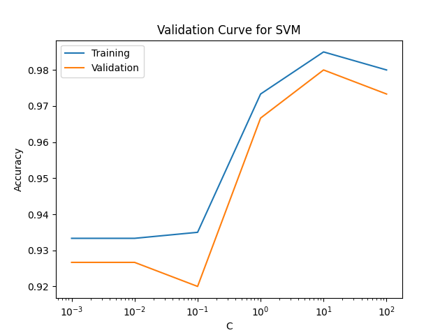

Interpretation:

Large gap between train and validation = overfitting.
Low performance on both = underfitting.

Learning Curve

Shows how model performance changes with training set size.

import numpy as np

import matplotlib.pyplot as plt

from sklearn.model_selection import learning_curve

from sklearn.svm import SVC

from sklearn.datasets import load_iris

X, y = load_iris(return_X_y=True)

model = SVC(kernel='linear')

train_sizes, train_scores, test_scores = learning_curve(

SVC(C=1.0), X, y, cv=5, train_sizes=np.linspace(0.1, 1.0, 5)

)

plt.plot(train_sizes, np.mean(train_scores, axis=1), label="Training")

plt.plot(train_sizes, np.mean(test_scores, axis=1), label="Validation")

plt.xlabel("Training Set Size")

plt.ylabel("Accuracy")

plt.title("Learning Curve for SVM")

plt.legend()

plt.show()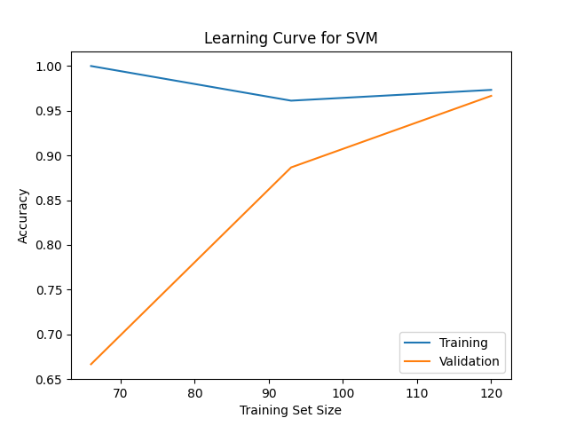

Use this to determine whether collecting more data would help or if the model is too complex.

Model Comparison

When multiple models perform similarly, you can use statistical techniques to compare them fairly.

Example comparing cross-validated scores:

from sklearn.model_selection import cross_val_score

from sklearn.linear_model import LogisticRegression

from sklearn.ensemble import RandomForestClassifier

from sklearn.svm import SVC

from sklearn.datasets import load_iris

X, y = load_iris(return_X_y=True)

model = SVC(kernel='linear')

lr = LogisticRegression(max_iter=200)

rf = RandomForestClassifier(random_state=42)

lr_scores = cross_val_score(lr, X, y, cv=5)

rf_scores = cross_val_score(rf, X, y, cv=5)

print("LR mean accuracy:", lr_scores.mean())

print("RF mean accuracy:", rf_scores.mean())

Best practice:
Choose the simplest model that performs adequately, not the most complex.

Overfitting and Underfitting

Behaviour	Description	Typical Fix
Underfitting	Model too simple, fails to capture patterns	Use a more complex model or add features
Overfitting	Model too complex, memorises training data	Regularise, simplify model, or gather more data

Visual check (conceptually):

Overfit → low training error, high test error
Underfit → high training and test error

Regularisation methods (like alpha in Ridge or C in SVM) directly control this balance.

Cross-Validation Best Practices

Always use stratified folds for classification.
Use cross-validation before reporting final performance.
Never tune hyperparameters on the test set, use a separate validation split or nested CV.
Use consistent random seeds for reproducibility.
For small datasets, prefer Leave-One-Out CV (LOOCV) or repeated k-fold.