Supervised Learning

Scikit-learn Basics

4 min read

Published Nov 17 2025, updated Nov 19 2025

ClusteringFeature EngineeringK-MeansLinear RegressionLogistic RegressionMachine LearningNumPyPythonRandom Forestsscikit-learnSupervised LearningUnsupervised Learning

Supervised learning is the foundation of most practical machine-learning systems.
In this paradigm, a model learns from labeled data, examples where both the inputs (X) and the desired outputs (y) are known.

The model’s goal is to discover the relationship between input features and target outputs so that it can make accurate predictions on new, unseen data.

Supervised learning is divided into two main categories:

Classification: Predicting discrete labels (e.g. “spam” or “not spam”).
Regression: Predicting continuous numeric values (e.g. predicting house prices).

Throughout this section, we’ll explore both tasks, their key concepts, and how to implement them efficiently using Scikit-learn.

The Supervised Learning Workflow

A typical supervised learning process involves:

Data Preparation - Split data into features (X) and labels (y), then divide into training and testing subsets.
Model Selection - Choose an appropriate algorithm for the problem (e.g. logistic regression, random forest).
Training - Fit the model to the training data using .fit(X_train, y_train).
Prediction - Apply the model to unseen data using .predict(X_test).
Evaluation - Measure performance using relevant metrics (accuracy, R², etc.).
Tuning and Validation - Refine hyperparameters and verify generalisation via cross-validation.

Classification

Classification problems involve assigning data points to one of a set of discrete categories. The model learns a decision boundary that separates these classes based on feature patterns.

Examples:

Spam filtering (spam / not spam)
Disease diagnosis (positive / negative)
Handwritten digit recognition (0–9)

Scikit-learn offers many classifiers, including:

LogisticRegression
KNeighborsClassifier
DecisionTreeClassifier
RandomForestClassifier
SVC (Support Vector Classifier)
GaussianNB (Naive Bayes)
GradientBoostingClassifier

All follow the same API pattern: fit → predict → evaluate.

Example: Logistic Regression on Iris Dataset

from sklearn.datasets import load_iris

from sklearn.model_selection import train_test_split

from sklearn.linear_model import LogisticRegression

from sklearn.metrics import accuracy_score, classification_report, confusion_matrix

# Load dataset

iris = load_iris()

X, y = iris.data, iris.target

# Split into train/test sets

X_train, X_test, y_train, y_test = train_test_split(X, y, test_size=0.2, random_state=42)

# Train model

model = LogisticRegression(max_iter=200)

model.fit(X_train, y_train)

# Predict

y_pred = model.predict(X_test)

# Evaluate

print("Accuracy:", accuracy_score(y_test, y_pred))

print("\nClassification Report:\n", classification_report(y_test, y_pred))

print("\nConfusion Matrix:\n", confusion_matrix(y_test, y_pred))

Output:

Accuracy: 1.0

Classification Report:

precision recall f1-score support

0 1.00 1.00 1.00 10

1 1.00 1.00 1.00 9

2 1.00 1.00 1.00 11

accuracy 1.00 30

macro avg 1.00 1.00 1.00 30

weighted avg 1.00 1.00 1.00 30

Confusion Matrix:

[[10 0 0]

[ 0 9 0]

[ 0 0 11]]

Notes:

Logistic regression is a baseline classification model, it performs well on linearly separable data.
max_iter ensures convergence for larger datasets.
The confusion matrix provides a detailed breakdown of prediction performance across classes.

Example: Decision Tree Classifier

from sklearn.datasets import load_iris

from sklearn.model_selection import train_test_split

from sklearn.metrics import accuracy_score

from sklearn.tree import DecisionTreeClassifier, plot_tree

import matplotlib.pyplot as plt

# Load dataset

iris = load_iris()

X, y = iris.data, iris.target

# Split into train/test sets

X_train, X_test, y_train, y_test = train_test_split(X, y, test_size=0.2, random_state=42)

# Train model

tree_clf = DecisionTreeClassifier(max_depth=3, random_state=42)

tree_clf.fit(X_train, y_train)

# Predict

y_pred = tree_clf.predict(X_test)

print("Accuracy:", accuracy_score(y_test, y_pred))

# Visualise tree

plt.figure(figsize=(10, 6))

plot_tree(tree_clf, feature_names=iris.feature_names, class_names=iris.target_names, filled=True)

plt.show()

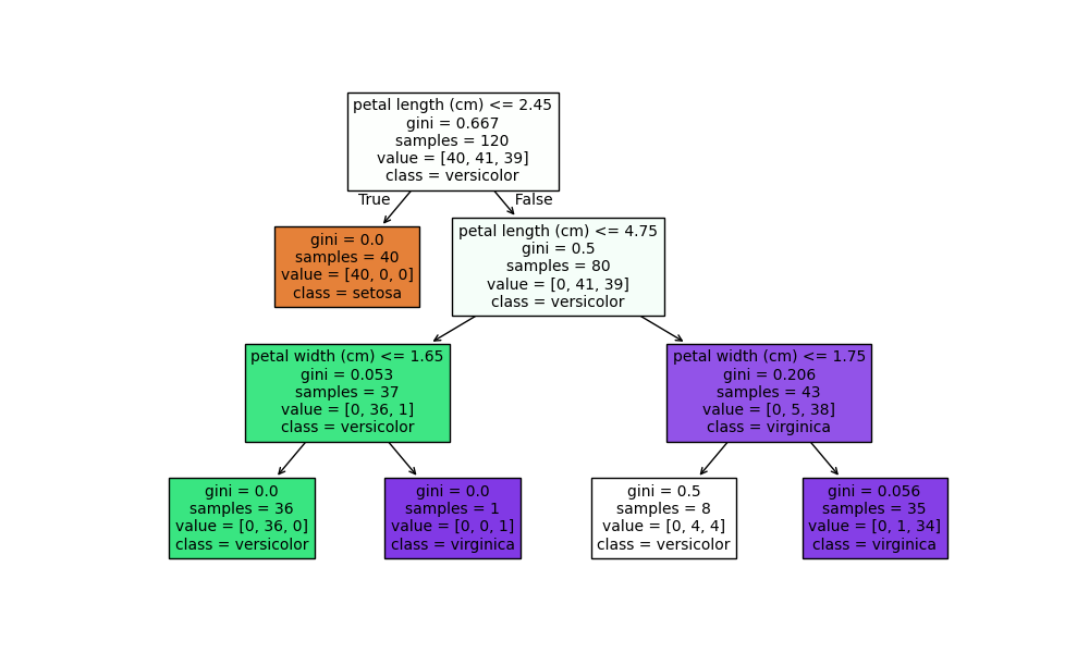
Notes:

Decision trees are intuitive and interpretable.
Limiting max_depth helps prevent overfitting.
Trees form the basis for powerful ensemble models like Random Forest and Gradient Boosting.

Key Classification Metrics

Metric	Description	Function
Accuracy	Percentage of correctly predicted samples	`accuracy_score`
Precision	Proportion of positive predictions that were correct	`precision_score`
Recall	Proportion of actual positives that were correctly predicted	`recall_score`
F1-score	Harmonic mean of precision and recall	`f1_score`
ROC-AUC	Trade-off between true and false positive rates	`roc_auc_score`

Example:

from sklearn.metrics import precision_score, recall_score, f1_score

print("Precision:", precision_score(y_test, y_pred, average='macro'))

print("Recall:", recall_score(y_test, y_pred, average='macro'))

print("F1 Score:", f1_score(y_test, y_pred, average='macro'))

Regression

Regression models predict continuous numeric values. Instead of predicting discrete labels, they estimate quantities.

Examples:

Predicting house prices
Estimating sales, temperature, or life expectancy

Common regression algorithms:

LinearRegression
Ridge, Lasso (regularised linear models)
DecisionTreeRegressor
RandomForestRegressor
SVR (Support Vector Regressor)
GradientBoostingRegressor

All regression estimators follow the same .fit() and .predict() pattern.

Example: Linear Regression

from sklearn.datasets import make_regression

from sklearn.linear_model import LinearRegression

from sklearn.model_selection import train_test_split

from sklearn.metrics import mean_squared_error, r2_score

# Generate synthetic regression data

X, y = make_regression(n_samples=200, n_features=2, noise=10, random_state=42)

X_train, X_test, y_train, y_test = train_test_split(X, y, test_size=0.2, random_state=42)

# Train model

reg = LinearRegression()

reg.fit(X_train, y_train)

# Predict

y_pred = reg.predict(X_test)

# Evaluate

print("Mean Squared Error:", mean_squared_error(y_test, y_pred))

print("R² Score:", r2_score(y_test, y_pred))

Notes:

R² measures how well the model explains the variance in the data.
MSE penalises larger errors more strongly, highlighting variance issues.
Linear regression assumes linear relationships and normally distributed residuals.

Example: Random Forest Regressor

from sklearn.datasets import make_regression

from sklearn.model_selection import train_test_split

from sklearn.metrics import mean_squared_error, r2_score

from sklearn.ensemble import RandomForestRegressor

# Generate synthetic regression data

X, y = make_regression(n_samples=200, n_features=2, noise=10, random_state=42)

X_train, X_test, y_train, y_test = train_test_split(X, y, test_size=0.2, random_state=42)

# Train Random Forest Regressor

rf = RandomForestRegressor(n_estimators=100, random_state=42)

rf.fit(X_train, y_train)

y_pred = rf.predict(X_test)

print("R²:", r2_score(y_test, y_pred))

print("MSE:", mean_squared_error(y_test, y_pred))

Notes:

Random forests average predictions from multiple trees to reduce variance.
They handle nonlinear data and mixed feature types well.
Generally robust with minimal tuning.

Regression Metrics

Metric	Description	Function
MAE (Mean Absolute Error)	Average absolute difference	`mean_absolute_error`
MSE (Mean Squared Error)	Average of squared differences	`mean_squared_error`
RMSE	Square root of MSE	`mean_squared_error(..., squared=False)`
R² Score	Proportion of variance explained	`r2_score`

Example:

from sklearn.metrics import mean_absolute_error, mean_squared_error, r2_score

mae = mean_absolute_error(y_test, y_pred)

mse = mean_squared_error(y_test, y_pred)

r2 = r2_score(y_test, y_pred)

print(f"MAE={mae:.2f}, MSE={mse:.2f}, R²={r2:.2f}")

Choosing and Comparing Models

There’s no one-size-fits-all algorithm, model selection depends on data size, feature relationships, and problem type.

Problem Type	Good Starting Model	Try Alternatives When...
Binary classification	Logistic Regression	Data is nonlinear → SVM, RandomForest
Multi-class classification	RandomForestClassifier	Dataset is large → GradientBoosting
Regression	LinearRegression	Data is nonlinear → RandomForest, SVR
Small dataset	KNN, DecisionTree	High-dimensional → Regularized models

Scikit-learn makes model comparison easy with cross-validation

Common Pitfalls

Skipping preprocessing - Unscaled features can bias distance-based algorithms (SVM, KNN).
Using accuracy on imbalanced data - Use precision, recall, or F1-score instead.
Forgetting to split data before training - Leads to data leakage and inflated performance metrics.
Overfitting trees or ensembles - Limit depth or tune hyperparameters via cross-validation.
Ignoring randomness - Always set random_state for reproducible results.