Working with Data

Scikit-learn Basics

3 min read

Published Nov 17 2025, updated Nov 19 2025

ClusteringFeature EngineeringK-MeansLinear RegressionLogistic RegressionMachine LearningNumPyPythonRandom Forestsscikit-learnSupervised LearningUnsupervised Learning

Every machine learning project begins with data, and how you manage that data largely determines the success of your models.

In Scikit-learn, all algorithms expect data in numeric, tabular form, typically represented as:

X → the feature matrix (inputs)
y → the target vector (labels or outputs)

This section covers how to:

Load data (from built-in datasets, generated data, or external files)
Explore and understand data structure
Split data into training and testing sets
Manage shapes, formats, and types so they align with Scikit-learn’s expectations

The Data Representation

Scikit-learn is designed to work primarily with:

NumPy arrays
pandas DataFrames
SciPy sparse matrices

These formats are used because they are fast, memory-efficient, and easy to manipulate.

Convention:

X is a 2D array of shape (n_samples, n_features)
y is a 1D array of shape (n_samples,)

For example:

import numpy as np

X = np.array([[1.2, 3.4], [2.3, 4.5], [3.1, 5.7]])

# 3 samples, 2 features

y = np.array([0, 1, 0])

# 3 target values

Many Scikit-learn utilities accept both NumPy arrays and pandas DataFrames:

import pandas as pd

df = pd.DataFrame(X, columns=['feature_1', 'feature_2'])

Internally, Scikit-learn converts these to NumPy arrays for computation.

Built-in Datasets

Scikit-learn provides a variety of small, well-known datasets for practice and demonstration.
They load instantly and are ideal for testing algorithms or learning workflows.

Common datasets:

Dataset	Function	Description
Iris	load_iris()	Flower classification (3 classes)
Wine	load_wine()	Wine chemical properties by cultivar
Breast Cancer	load_breast_cancer()	Binary classification
Digits	load_digits()	Handwritten digits (0–9)
Diabetes	load_diabetes()	Regression dataset
California Housing	fetch_california_housing()	House price regression

Example: Loading the Iris Dataset

from sklearn.datasets import load_iris

iris = load_iris()

X = iris.data

y = iris.target

print("Feature names:", iris.feature_names)

print("Target names:", iris.target_names)

print("Data shape:", X.shape)

Output:

Feature names: ['sepal length', 'sepal width', 'petal length', 'petal width']

Target names: ['setosa' 'versicolor' 'virginica']

Data shape: (150, 4)

Note:

load_iris() returns a Bunch object, a dictionary-like container with attributes (.data, .target, .feature_names, etc.)
Convert to pandas for easier exploration:

import pandas as pd

df = pd.DataFrame(X, columns=iris.feature_names)

df['target'] = iris.target

Generating Synthetic Data

For testing or demonstrations, you can generate synthetic datasets with controlled properties.
These functions are especially useful for experimenting with algorithms without needing external data.

Examples:

make_classification() - creates random classification problems
make_regression() - creates regression problems
make_blobs() - creates clustered data
make_moons(), make_circles() - create 2D toy datasets for visualisation

Example: Synthetic Regression Data

from sklearn.datasets import make_regression

import matplotlib.pyplot as plt

X, y = make_regression(n_samples=100, n_features=1, noise=10, random_state=42)

plt.scatter(X, y)

plt.xlabel("Feature")

plt.ylabel("Target")

plt.title("Synthetic Regression Data")

plt.show()

scikit learn synthetic regression data chart

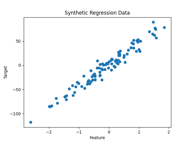
These synthetic datasets are invaluable for:

Benchmarking algorithms
Testing preprocessing pipelines
Visualising model behaviour

Loading External Data

Most real-world data comes from files, typically CSVs, Excel sheets, or databases. Scikit-learn doesn’t directly handle file I/O, instead, you’ll use pandas for that step.

Example: Loading a CSV with pandas

import pandas as pd

data = pd.read_csv('customer_data.csv')

# features

X = data[['age', 'income', 'purchases']]

# target label

y = data['churn']

Then, you can pass X and y directly to Scikit-learn models:

from sklearn.ensemble import RandomForestClassifier

model = RandomForestClassifier()

model.fit(X, y)

Note:

Ensure all input data is numeric, models cannot handle text directly.
Categorical features must be encoded.

Splitting Data for Training and Testing

When building a model, always split your dataset into training and testing subsets.
This allows you to train the model on one portion and evaluate it on unseen data to measure generalisation.

Scikit-learn provides train_test_split for this:

from sklearn.model_selection import train_test_split

X_train, X_test, y_train, y_test = train_test_split(

X, y, test_size=0.2, random_state=42

)

test_size=0.2 - 20% test data
random_state=42 - ensures reproducibility
For classification tasks, use stratify=y to maintain class balance (the proportion of each class in y will be (as closely as possible) the same in both the training and testing datasets):

train_test_split(X, y, test_size=0.2, stratify=y, random_state=42)

Keep your test data untouched until final evaluation. Avoid using it for feature scaling or tuning.

Data Shapes and Sanity Checks

Before training, it’s important to verify that your data is shaped correctly.

Common Issue	Symptom	Solution
Wrong shape	“Found array with dim 3”	Ensure `X` is 2D: `X.reshape(-1, n_features)`
Mismatched samples	“Input variables have inconsistent numbers of samples”	Check that `len(X) == len(y)`
Missing values	Model errors or NaNs in input	Handle via `SimpleImputer`