Categorical plot
Seaborn basics
2 min read
Published Oct 7 2025
Guide Sections
Guide Comments
seaborn.catplot() is a high-level figure-level function for creating categorical plots in Seaborn.
It combines the features of several categorical plotting functions — like:
sns.stripplot()sns.swarmplot()sns.boxplot()sns.violinplot()sns.barplot()sns.countplot()
…and adds faceting support (multiple subplots based on data subsets).
Essentially, catplot() = categorical plot + easy subplotting (faceting).
Syntax:
Parameters:
data= DataFrame containing your datax,y= Categorical and numerical variableshue= Adds subgroups (coloured)kind= Type of categorical plot to draw ("strip", "swarm", "box", "violin", "bar", "count", "boxen")col,row= Variables for faceting (creating subplots)order,hue_order= Category orderingpalette= Colour schemeheight= Height (in inches) of each subplotaspect= Width = height × aspectorient= "v" (vertical) or "h" (horizontal)dodge= Separate hue categorieslegend= Show or hide legendmargin_titles= Add titles on the edges of facets
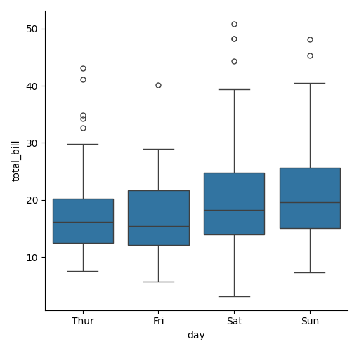
Basic example
Creates a boxplot showing the distribution of total_bill for each day.
Kinds of categorical plots
Kind | What It Shows | Equivalent Function |
"strip" | Individual data points (with possible jitter) | sns.stripplot() |
"swarm" | Non-overlapping points | sns.swarmplot() |
"box" | Summary statistics (quartiles, median, outliers) | sns.boxplot() |
"violin" | Distribution + density + quartiles | sns.violinplot() |
"boxen" | Enhanced boxplot for large datasets | sns.boxenplot() |
"bar" | Aggregated values (mean + CI) | sns.barplot() |
"count" | Counts of each category | sns.countplot() |
You can switch kind to change the plot type — no need to rewrite code.
Faceting: split data into subplots
Faceting = multiple subplots based on different subsets of your data.
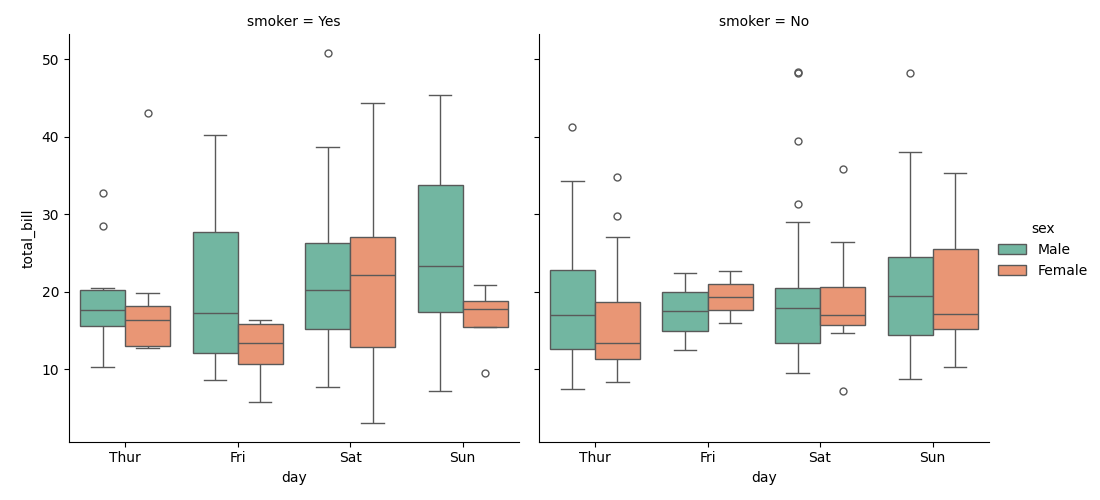
Facet by Column:
Creates one subplot for smokers and one for non-smokers.
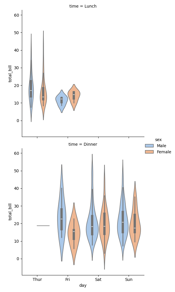
Facet by Row:
One row for Lunch and one for Dinner.
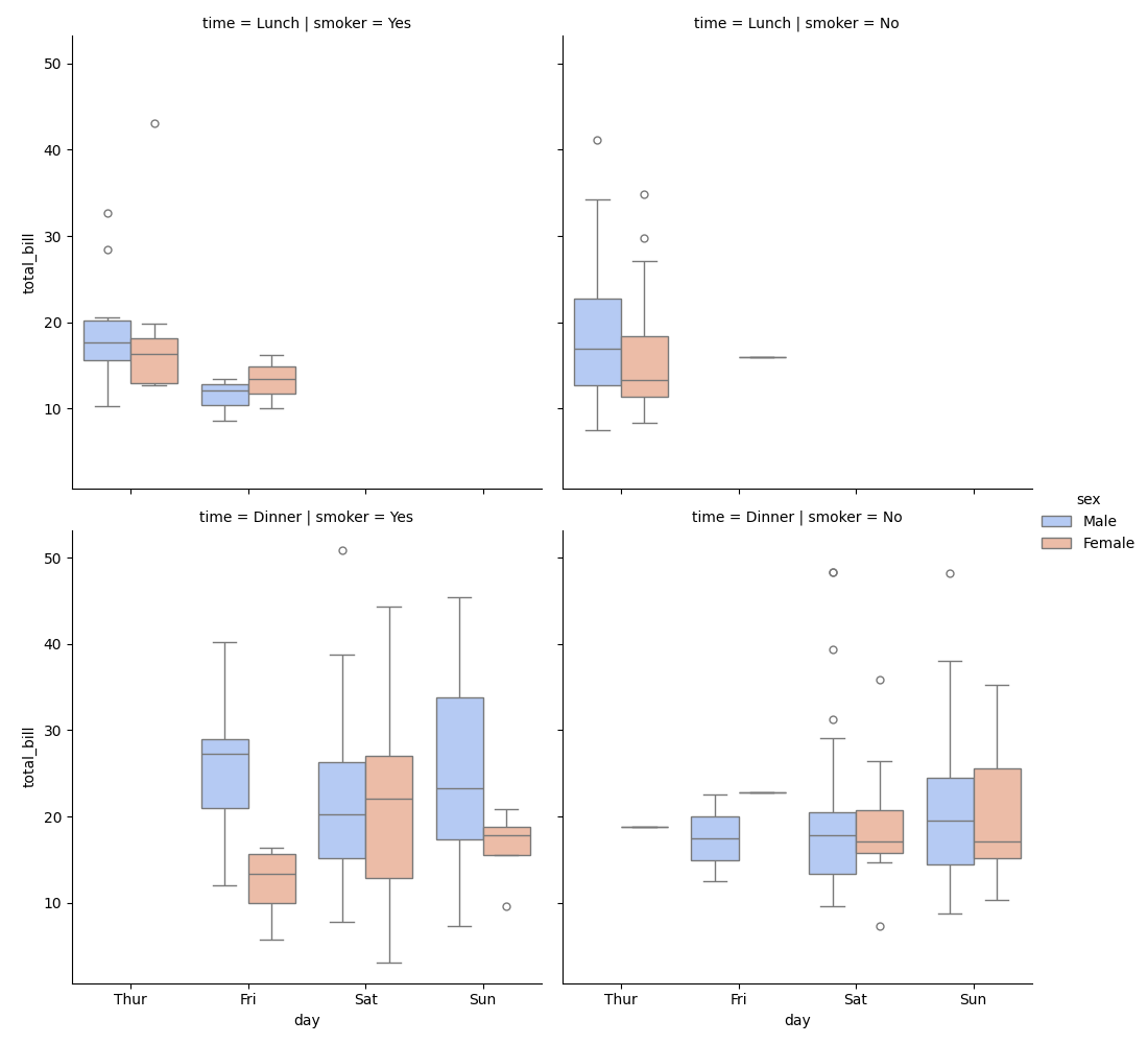
Facet by both row and column
Grid of subplots by both smoker and time.
Products from our shop
Docker Cheat Sheet - Print at Home Designs

Docker Cheat Sheet Mouse Mat

Docker Cheat Sheet Travel Mug

Docker Cheat Sheet Mug
Vim Cheat Sheet - Print at Home Designs

Vim Cheat Sheet Mouse Mat

Vim Cheat Sheet Travel Mug

Vim Cheat Sheet Mug

SimpleSteps.guide branded Travel Mug

Developer Excuse Javascript - Travel Mug

Developer Excuse Javascript Embroidered T-Shirt - Dark

Developer Excuse Javascript Embroidered T-Shirt - Light

Developer Excuse Javascript Mug - White

Developer Excuse Javascript Mug - Black

SimpleSteps.guide branded stainless steel water bottle

Developer Excuse Javascript Hoodie - Light
