Clustered Heatmap

seaborn.clustermap() creates a clustered heatmap — a combination of:

• A heatmap (coloured grid of values), and
• Hierarchical clustering on both rows and columns.

It automatically reorders rows and columns to group similar patterns together, and draws dendrograms (tree diagrams) showing the clustering structure.

It’s commonly used in:

• Gene expression analysis
• Feature correlation exploration
• Pattern detection in any tabular numeric data

Syntax:

sns.clustermap(    data,    *,    pivot_kws=None,    method='average',    metric='euclidean',    z_score=None,    standard_scale=None,    figsize=None,    cmap=None,    center=None,    robust=False,    annot=None,    fmt=".2g",    annot_kws=None,    linewidths=0,    linecolor='white',    cbar_pos=(0.02, 0.8, 0.05, 0.18),    cbar_kws=None,    mask=None,    dendrogram_ratio=0.2,    colors_ratio=0.03,    cbar_pos_ratio=0.15,    tree_kws=None,    row_cluster=True,    col_cluster=True,    row_linkage=None,    col_linkage=None,    xticklabels=True,    yticklabels=True,    vmin=None,    vmax=None,    **kwargs)

Parameters:

• data = 2D data (DataFrame or matrix)
• method = Clustering algorithm: "single", "complete", "average", "ward", etc.
• metric = Distance measure: "euclidean", "correlation", "cityblock", etc.
• z_score = Normalise rows (0) or columns (1) to z-scores
• standard_scale = Scale rows (0) or columns (1) between 0 and 1
• cmap = Colour map for the heatmap
• center = Value to centre the colourmap
• annot = Display numerical values in cells
• row_cluster / col_cluster = Enable/disable clustering on rows or columns
• row_linkage, col_linkage = Precomputed linkage matrices for custom clustering
• xticklabels, yticklabels = Show/hide or customise labels
• figsize = Size of the entire clustered plot
• tree_kws = Arguments for dendrogram styling

Basic example

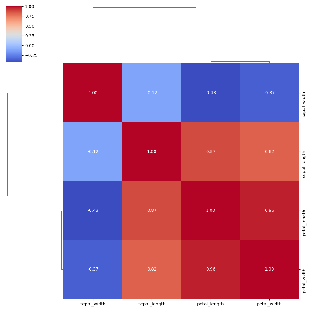
import seaborn as snsimport matplotlib.pyplot as plt​iris = sns.load_dataset("iris")corr = iris.corr(numeric_only=True)​sns.clustermap(corr, cmap="coolwarm", annot=True)plt.show()

Displays a correlation matrix clustered by similarity. Similar variables are grouped together with dendrograms on top and left.

Customise color palette

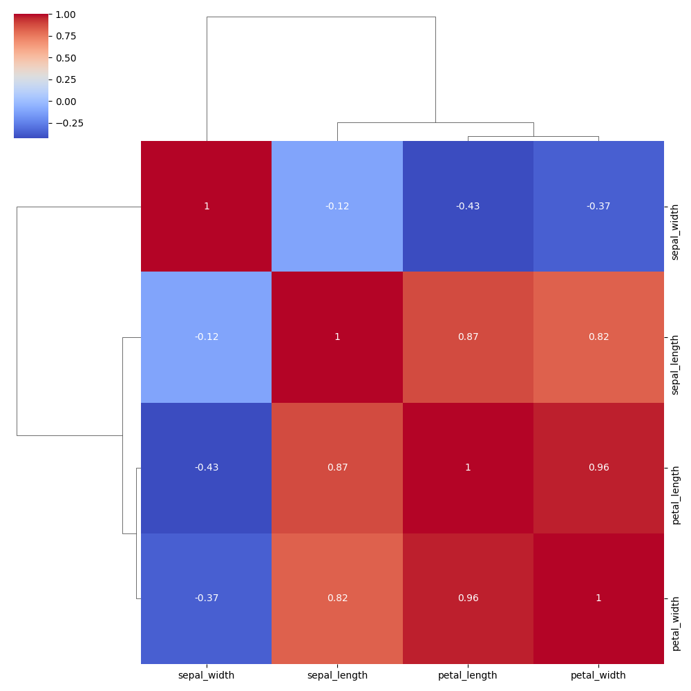
import seaborn as snsimport matplotlib.pyplot as plt​iris = sns.load_dataset("iris")corr = iris.corr(numeric_only=True)​sns.clustermap(corr, cmap="viridis", annot=True)plt.show()

You can use any Matplotlib or Seaborn colourmap ("mako", "crest", "rocket", etc.).

Normalise data (z-score)

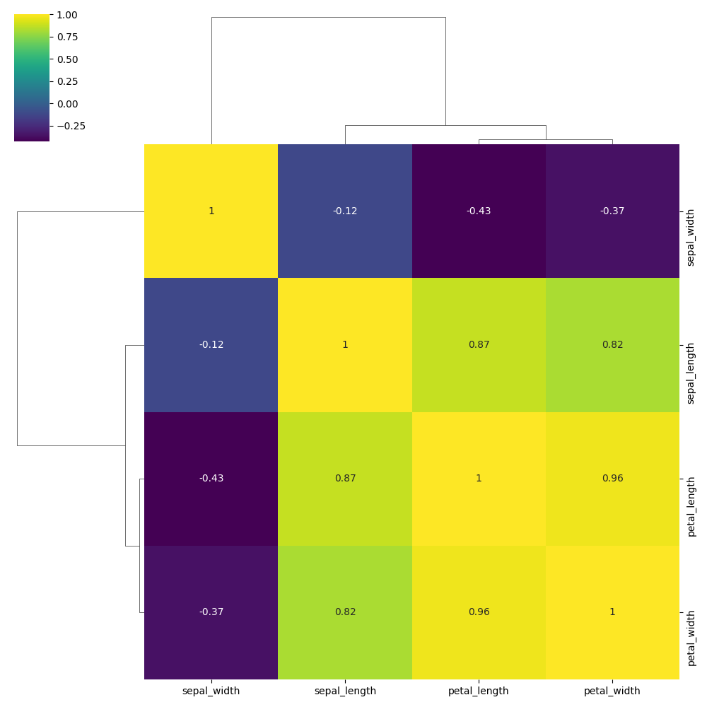
import seaborn as snsimport matplotlib.pyplot as plt​iris = sns.load_dataset("iris")corr = iris.corr(numeric_only=True)​sns.clustermap(corr, cmap="coolwarm", z_score=0)plt.show()

Normalises data by rows to z-scores (mean = 0, std = 1). Use z_score=1 to normalise by columns.

Disable clustering

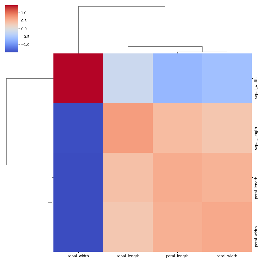
Keeps the data order fixed along the chosen axis.

No Row Clustering:

import seaborn as snsimport matplotlib.pyplot as plt​iris = sns.load_dataset("iris")corr = iris.corr(numeric_only=True)​sns.clustermap(corr, row_cluster=False, cmap="coolwarm")plt.show()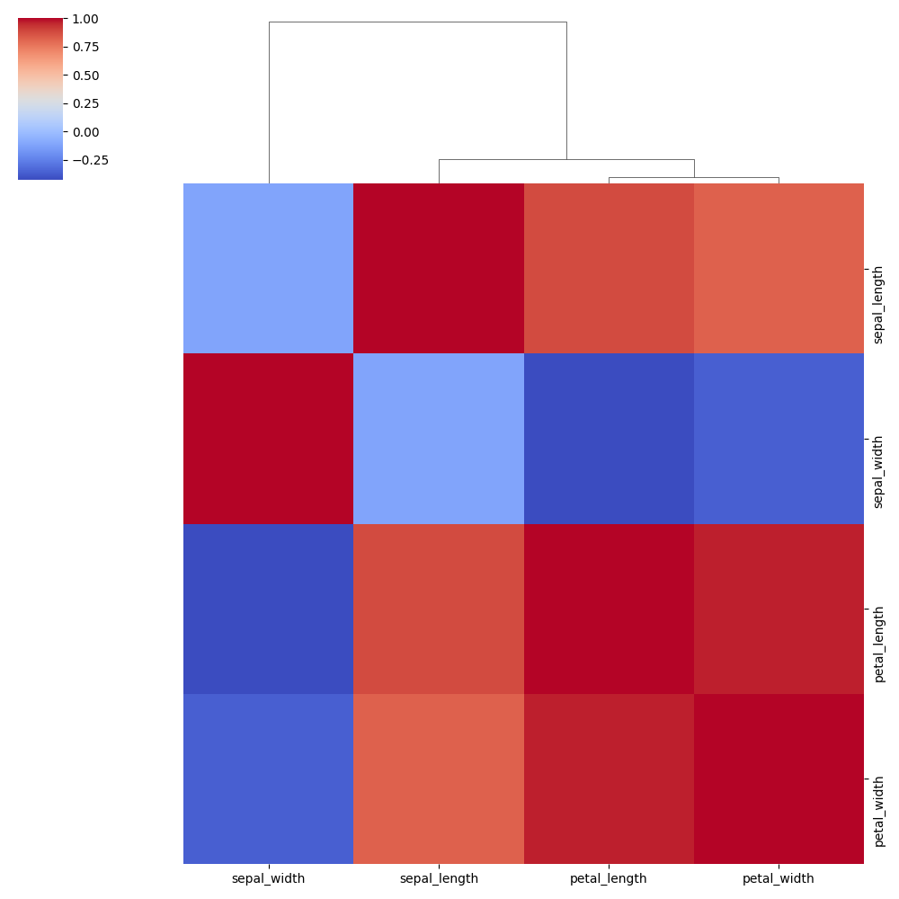

No Column Clustering:

import seaborn as snsimport matplotlib.pyplot as plt​iris = sns.load_dataset("iris")corr = iris.corr(numeric_only=True)​sns.clustermap(corr, col_cluster=False, cmap="coolwarm")plt.show()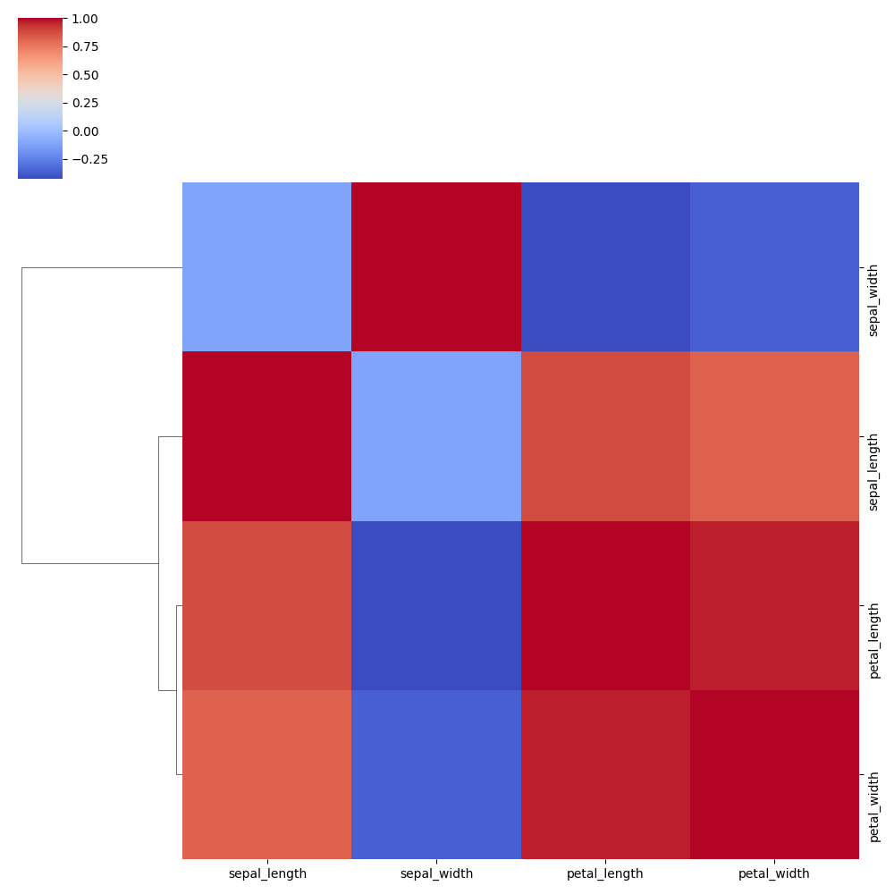

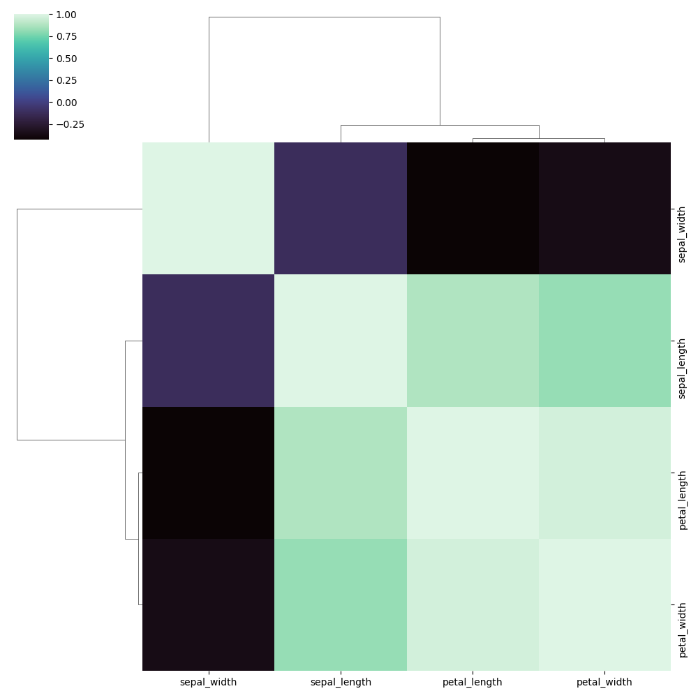
Change clustering method and distance

import seaborn as snsimport matplotlib.pyplot as plt​iris = sns.load_dataset("iris")corr = iris.corr(numeric_only=True)​sns.clustermap(corr, method="ward", metric="euclidean", cmap="mako")plt.show()

Controls how clusters are formed:

• method: linkage type ("ward", "average", "complete", etc.)
• metric: distance measure ("euclidean", "cosine", "correlation", etc.)

Add annotations

import seaborn as snsimport matplotlib.pyplot as plt​iris = sns.load_dataset("iris")corr = iris.corr(numeric_only=True)​sns.clustermap(corr, cmap="coolwarm", annot=True, fmt=".2f")plt.show()

Displays the numeric values inside each cell. Great for small matrices (e.g., correlation heatmaps).